Motivation #
Throughout my Bachelor’s and Master’s in Computer Science, I have listened to many lecturers talk about the Transformer architecture. But just listening never really teaches you how something works. You have to do that yourself. And that was my main motivation for finally implementing the Transformer. Reading Attention Is All You Need (certainly not for the first time), but for the first time with the goal of doing it myself led me to understand at a deeper, more intuitive level. Here is what I learned; if you are on a similar path, I hope you find this useful. I also link to the many great resources that helped me understand this topic better - be sure to check them out!
Note: I published the code on github (click) which includes a notebook to play around with.
Tokenization and Dataset #
As described in the original Transformer paper:
“We trained on the standard WMT 2014 English-German dataset consisting of about 4.5 million sentence pairs. Sentences were encoded using byte-pair encoding [3], which has a shared source-target vocabulary of about 37,000 tokens.” (Section 5.1)
In classic paper style, just a single sentence, but to find the correct dataset, to learn about byte-pair encoding and to select the tokenization scheme took me quite some time… :). I wanted to use the original WMT 2014 dataset, though if you have less available compute, then the Multi30k dataset is a good alternative.
Either way, I found the WMT 2014 dataset already preprocessed into English–German text pairs here. We can’t pass the raw sentences as strings into any model, so the first step is always Tokenization. The process behind Tokenization is the aforementioned byte-pair encoding which iteratively merges the most frequent token pair into a single new token. I don’t want to go super deep into this, and instead just point to this amazing video from Andrej Karpathy:
Around 90 minutes in, he briefly mentions SentencePiece from Google which he says is a bit more clunky than the now more popular alternative tiktoken from OpenAI, but I figured using SentencePiece would be closer to the AIAYN regime, and went with it.
And it turns out, it’s actually straightforward to get working. I will share it here directly, because I had a hard time finding any other reimplementation that uses it.
from datasets import load_dataset
import sentencepiece as spm

ds = load_dataset("stas/wmt14-en-de-pre-processed", "ende")
assert "train" in ds
train_ds = ds["train"]

with open("bpe_train_corpus.txt", "w", encoding="utf-8") as f:
    for example in train_ds:
        german = example["translation"]["de"]
        english = example["translation"]["en"]
        f.write(german + "\n")
        f.write(english + "\n")

spm.SentencePieceTrainer.Train(
    input="bpe_train_corpus.txt",
    model_prefix="ende_bpe",
    vocab_size=37000,
    model_type="bpe",
    character_coverage=1.0,
    input_sentence_size=2000000,
    pad_id=0,
    unk_id=1,
    bos_id=2,
    eos_id=3,
)
Because we are dealing with English–German, we can set the character_coverage to 1 (which means the Tokenizer will cover all characters) and we also set our special tokens manually. We need padding for efficient batching, the bos and eos tokens to mark beginning and end of sentences, and the unknown token in case any subword is not covered by the trained vocabulary. This could be typos, or unexpected foreign characters.
That’s it. Tokenizer “already” done training. The output is a .model and .vocab file, the latter being a reference to investigate.
Transformer Architecture #
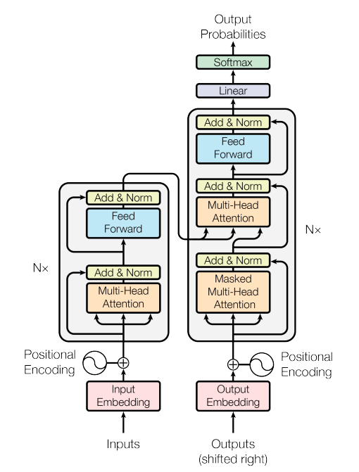
I have seen this architecture figure many times… but in my opinion, just staring at this architecture and trying to understand how it works, and more importantly, why you would come up with this, doesn’t really work. Instead, I would suggest reading this article from Jay Alammar. It’s an amazing brief history on Seq2Seq translation and makes it clear why the concept of “Attention” emerged.
Here is what I got away from it: Early work just used the Encoder-Decoder stack. The encoder encodes the original sequence into an embedding, and the decoder uses it to produce the translation. The pitfall of this is long sentences (How much information can you store about a sentence in one fixed length vector?)
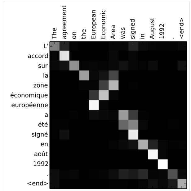
Thus the idea behind attention was born. Instead of passing one single embedding (hidden state in RNN world), we pass all! And the decoder uses a scoring mechanism to know how strongly it should attend to each hidden state for the respective decoding step (just by taking the weighted sum of the respective hidden states!). Why is this so useful - why can’t the decoder produce output token #5 just not always use the encoding of input token #5 for the translation? Check out the attention-map below. The model needs to translate European Economic Area to zone économique européenne - the reverse.
Embeddings #
Back to the Transformer architecture now. What happens off screen, is the aforementioned tokenization: The sentence gets encoded to a sequence of IDs. These IDs are then fed through the embedding layer, which encodes each ID as a 512-dimensional vector.
“Similarly to other sequence transduction models, we use learned embeddings to convert the input tokens and output tokens to vectors of dimension dmodel.” (Section 3.4)
Then positional encodings are added, which are needed for each word to have a representation of where it appears in the sequence. If we did not do that, to the model the sentences “The cat loves milk” and “The milk loves cat” would look identical. There can be a lot more said about positional encodings, but I did not want to spend too much time on them myself.
“Since our model contains no recurrence and no convolution, in order for the model to make use of the order of the sequence, we must inject some information about the relative or absolute position of the tokens in the sequence. To this end, we add “positional encodings” to the input embeddings at the bottoms of the encoder and decoder stacks. The positional encodings have the same dimension dmodel as the embeddings, so that the two can be summed.” (Section 3.5)
Encoder #
Note: I will be ignoring residual connections, layer norm and dropout. They are classic ML techniques that don’t add much to conceptual understanding but are required for good results. Check them out in the code or paper instead.
“The encoder is composed of a stack of N = 6 identical layers. Each layer has two sub-layers. The first is a multi-head self-attention mechanism, and the second is a simple, positionwise fully connected feed-forward network.” (Section 3.1)
This sentence describing the sub-layers is the heart of the Transformer architecture. First, there is self-attention.
Self-Attention #
“We call our particular attention “Scaled Dot-Product Attention” (Figure 2). The input consists of queries and keys of dimension dk, and values of dimension dv. We compute the dot products of the query with all keys, divide each by √ dk, and apply a softmax function to obtain the weights on the values.” (Section 3.2)
This is now the heart of it. First, intuition. Why attention in the first place? Attention is used to transport information from one place in the sentence to the next. Think of the following sentence: “The man was hungry because he had not eaten.” Now “he” is most likely a token (or rather " he" ;)). But “he” also relates to the man, so the model needs to relate these two and then move some of the information of the man to the “he” token. What kind of information? Could be the fact that the man is hungry. Mathematically, this moving of information is defined as the following:
$$ \text{Attention}(Q, K, V) = \text{softmax}\left(\frac{QK^T}{\sqrt{d_k}}\right)V $$Now we can think of the “he” from the example sentence before as our query. For this we compute a query vector. For all words in the sentence we compute a key vector and a value vector (and put them into the matrices K and V). Then we take the dot product of the query vector with all key vectors from the key matrix. This is our similarity score, so we know how much information of each word (including “he” itself), we want. We softmax to get a probability distribution and then multiply the similarity score that each word has to “he”, with the value vector of the respective word. That’s all there is to it! And of course, we do all of this in matrix form, in parallel for all words. The equation also normalizes the softmax, but in Łukasz’ words, this is an implementation detail and not at all needed to understand the gist of attention.
Multi-Head Attention #
“Instead of performing a single attention function with dmodel-dimensional keys, values and queries, we found it beneficial to linearly project the queries, keys and values h times with different, learned linear projections to dk, dk and dv dimensions, respectively. On each of these projected versions of queries, keys and values we then perform the attention function in parallel, yielding dv-dimensional output values.” (Section 3.2)
In the paper this is worded… paperly, but the essence is very simple to grasp again. Instead of doing one of these attention computations, we do several in parallel. Because this then allows each attention head (that is to say each set of learned linear transformations) to attend to / focus on something different. We concatenate all of the results and multiply with a learned output transformation before passing it to the next layer.
And this is attention. In the first Encoder Layer, we use the embedded inputs as our values to calculate the query, key and value matrices, and in subsequent layers, the output from the previous one.
Further Resources:
- The Illustrated Transformer
- The Attention Chapter from this course on Transformers
- Łukasz Kaiser talk (really worth a watch)
Feed-Forward Layer #
As much as the self-attention layers are about transporting information, they cannot create new features. That’s what we need the linear layers for. In the Transformer stack, these are just your standard two layers with a RELU-non linearity in between.
$$ \text{FFN}(x) = \max(0, xW_1 + b_1)W_2 + b_2 $$Decoder #
The decoder’s architecture closely mirrors that of the encoder. During inference, it generates the target sequence one token at a time, always conditioning on the tokens it has already produced—starting with the special start-of-sequence (<bos>) token. These undergo the same embedding as in the encoder.
Self-attention largely remains the same. However, during training, we take advantage of teacher forcing: the entire target sequence is available, so the model learns to predict token i+1 given tokens 1...i, for all positions in parallel. This is much more efficient than generating tokens one by one. To ensure the model cannot “cheat” by looking ahead, we apply a mask in the self-attention mechanism so that, when predicting position i+1, the decoder can only attend to tokens at positions less than or equal to i.
Before the Feed-Forward layer there is an additional block: Encoder-Decoder attention. Mechanically it works just like the self-attention layer before, but the key and value matrices are computed with the output of the final encoder layer. This then allows the Decoder to integrate information from the full encoded input sequence in each of the six decoder blocks.
Projection #
After the Decoder stack, the output is projected back to the embedding space and a final softmax is applied to get the probability distribution over all tokens. Again - easy, especially if you have worked with classification tasks before.
Training #
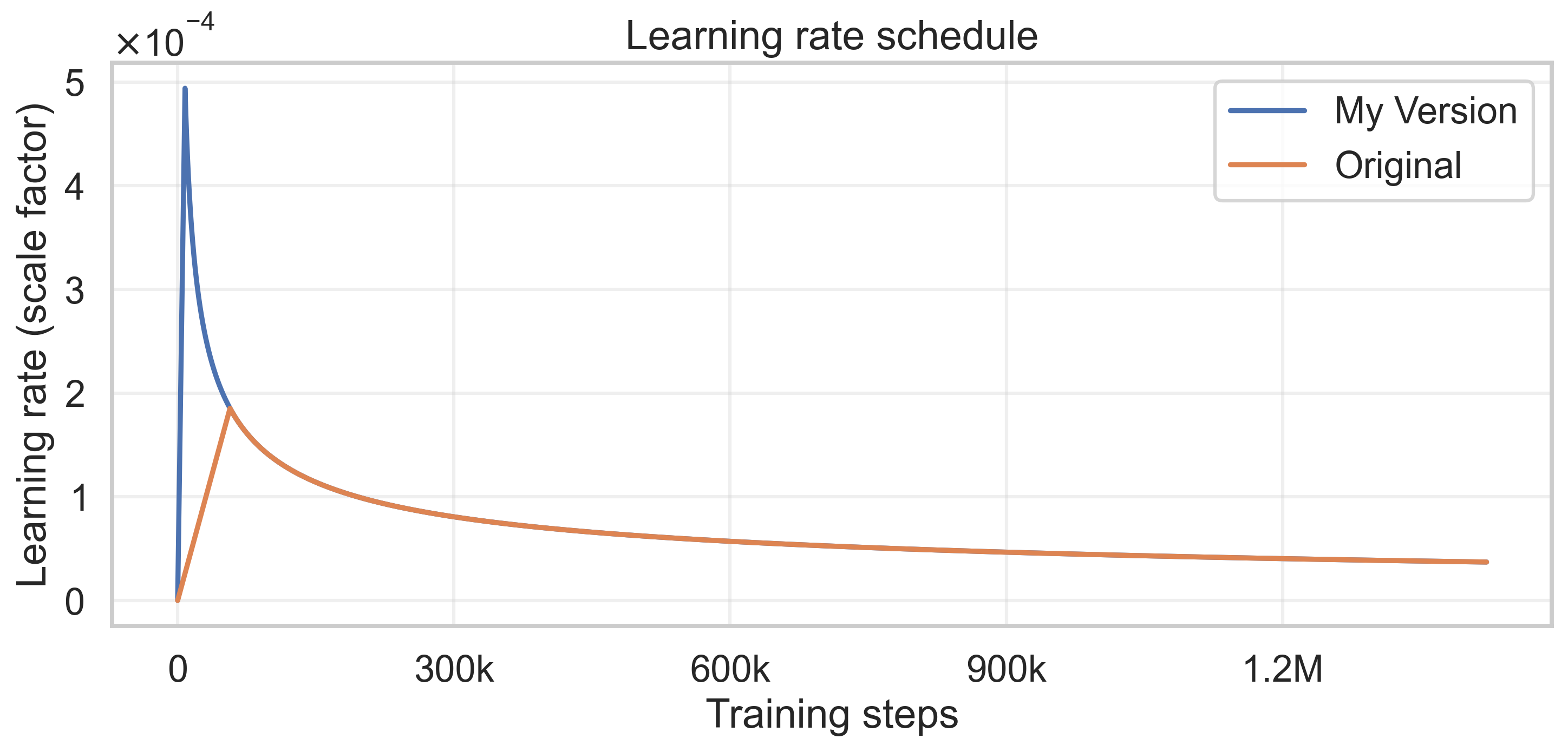
To train, I made some adjustments. One, I was only able to fit a batch size of 32 in memory, whereas the paper used a much larger set of examples. Second, I did not scale the warmup_steps of the LR schedule appropriately and ended up with a much shorter warmup window and higher initial LR.
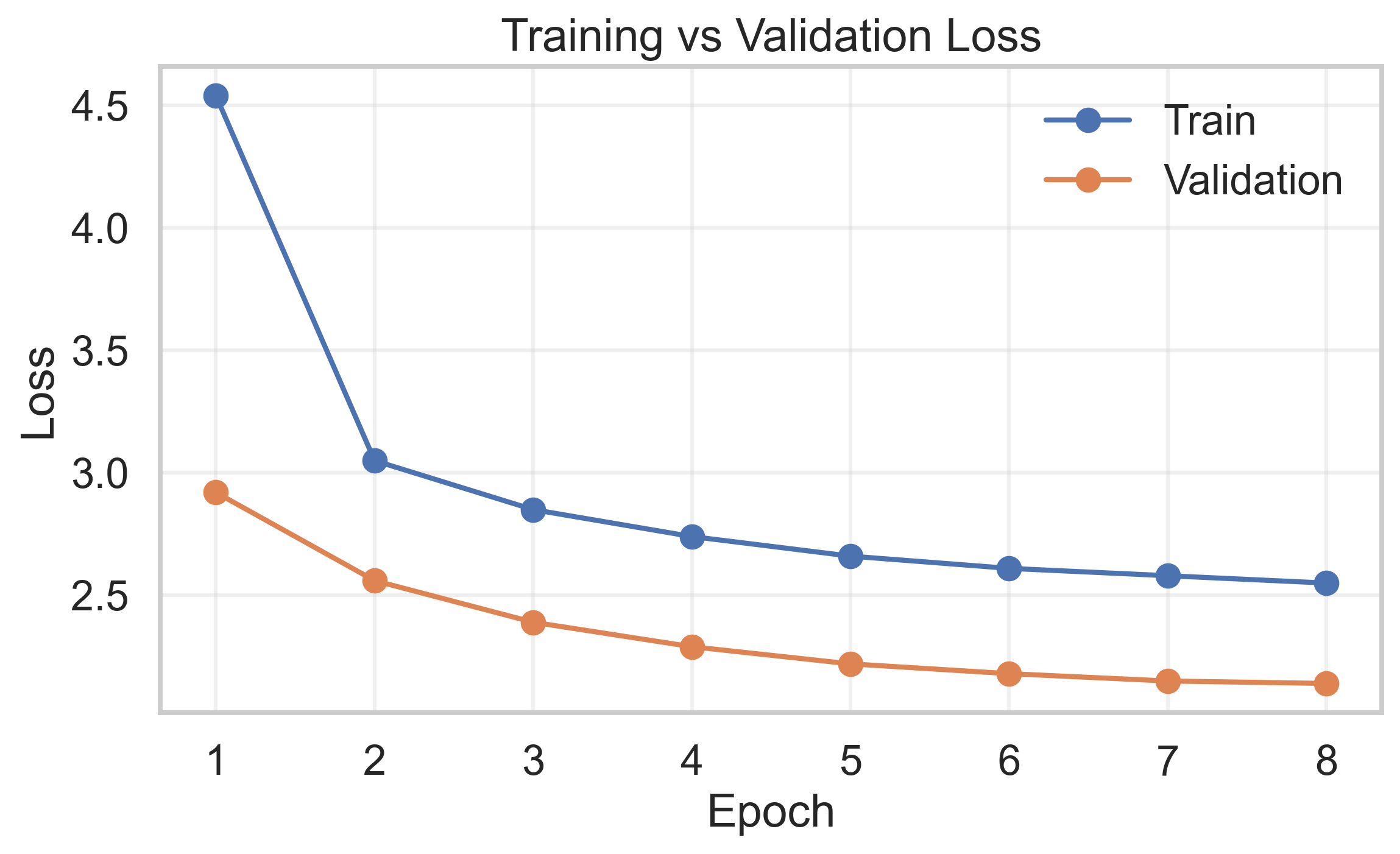
For training, I rented a single RTX 3090 GPU on runpod which makes it extremely easy to get up and running (sign up here). Renting an RTX 3090 costs 0.47$/hr and I trained for a total of 8 epochs, with each epoch taking around 4 hours. Of course, I could have trained for longer, but at this point the performance was already pretty good, as I will show in a second.
Inference #
After all this work it’s now time to reap the rewards. How does the model perform? For inference there are two ways of picking the next token: greedy and beam search. The greedy version is easy to explain: Here, we always append the one token that has the highest probability peak after softmax.
Beam search is a bit more sophisticated, but also not hard to understand. Instead of just taking the word with the highest probability, we save the k paths with the highest total probability. Instead of just predicting the next token, given our decoded sequence so far, we predict the k most likely tokens, for each of the k paths already chosen, and take the k ones of these that have the highest total probability.
Running the evaluation on the test set showed the BLEU-score, the prevalent metric for Machine Translation tasks, improving when using Beam Search.
| Model | Decoding Strategy | Dataset | BLEU |
|---|---|---|---|
| Transformer (Vaswani et al.) | Beam search | WMT14 EN–DE | 27.30 |
| My implementation | Greedy | WMT14 EN–DE | 26.20 |
| My implementation | Beam search | WMT14 EN–DE | 27.45 |
Check out these one, two to read more about how BLEU is computed
Closing Thoughts #
This was incredibly fun and rewarding to have a decent working model in the end. The whole process taught me quite a bit about the internals, specifically about self-attention that I had before regularly glossed over. I feel a lot more confident going further now, into actual LLM territory. My next project here will probably be related to the GPT family.